Table of Contents
R plots
Box plots
An user guide to walk through data visualization by box plot in R.
Please see the tutorials for more details.
One batch with replicates
Single batch boxplot tutorials
Sample input
R script
- single-batch_boxplot.R
# Aim: This R script is about making single batch boxplot.

# Data Description: One batch with replicates
# - sample1.xlsx
#   - Sheet1: Contains raw data across two columns: `Strain` and `Value`. Each strain includes 20 replicates.
#   - Sheet2: Contains the statistical test result (Tukey's HSD).
#
# Output (both pdf and png format):
# - Version 1: Displays all data points using a single color.
# - Version 2: Colors the data points by strain and adds statistical significance group labels at the top.
#---------------------------------------------------------------------------------------------------------------

### Step 0, Check packages

# Required packages
packages <- c("ggplot2", "readxl")

# Check and install required packages
for (pkg in packages) {
  if (!requireNamespace(pkg, quietly = TRUE)) {
    install.packages(pkg, repos = "https://cloud.r-project.org")
  }
}

#---------------------------------------------------------------------------------------------------------------

### Step 1. Configuration

## Set up a dedicated working directory to store your raw files and output plots.

# working directory
working_path = "/scratch/hychang/R_wd/Rana001/Rana001.01/single-batch/"

# input data located directory
input_path = "/scratch/hychang/R_wd/Rana001/Rana001.01/single-batch/"

# output folder for storing plots
output_path = "/scratch/hychang/R_wd/Rana001/Rana001.01/single-batch/plots/"

## Set Input and output

# File name of the raw data table, including the file extension
input_file_raw = "sample1.xlsx"

# Worksheet name of the raw data table
input_sheet_raw =  "Sheet1"

# (Optional) File name of the statistical test result table, including the file extension
input_file_stat = "sample1.xlsx"

# (Optional) Worksheet name of the statistical test result table
input_sheet_stat = "Sheet2"

# Column names in the input data
x_column = "Strain"
y_column = "Value"

# Column name of statistical significance group letters, skip if the statistical test not available
stat_column = "groups"

# Output file names of the figures, including the file extension
output_file_1 = "single-batch_v1.pdf"
output_file_2 = "single-batch_v2.pdf"
output_file_3 = "single-batch_v1.png"
output_file_4 = "single-batch_v2.png"

# Set up a dedicated working directory to store your raw files and output plots.
dir.create(working_path, recursive = TRUE, showWarnings = FALSE)
dir.create(input_path, recursive = TRUE, showWarnings = FALSE)
dir.create(output_path, recursive = TRUE, showWarnings = FALSE)

## Setting figure parameters

# the names of x and y axis
x_lab = "Strain"
y_lab = "Value"

# y axis range and breaks
y_range = c(0, 7)
y_breaks = c(0, 2, 4, 6)

# font size of x and y axis title (axis label)
axis_title_size = 16

# font size of x and y axis text (tick label)
axis_text_size = 14

# sample ordering
x_order = c("A", "B", "C")

# size of data points
point_size= 2

# box size
box_size= 0.4

# use a single color for all data points
color_single = c("#003175")

# use multiple colors for the data points; the number of colors should match the number of samples
color_multiple = c(c("#1B9E77", "#D95F02", "#7570B3"))

## Export setting
pdf_width = 6
pdf_height = 4
png_width = 600
png_height = 400

#---------------------------------------------------------------------------------------------------------------

### Step 2. Setup and Import data

# Set working directory
setwd(working_path)

# load packages
library(readxl)
library(ggplot2)

# Import raw data
df1= read_xlsx(file.path(input_path, input_file_raw), sheet = input_sheet_raw)

# (Optional) Import statistical test result. Skip this step if you don't have the results.
df2= read_xlsx(file.path(input_path, input_file_stat), sheet = input_sheet_stat)

# Sample ordering
df1[[x_column]] = factor(df1[[x_column]], levels = x_order)
df2[[x_column]] = factor(df2[[x_column]], levels = x_order) # skip this if df2 not available

# Display the data frame and view its dimensions (number of rows and columns).
df1; dim(df1)
df2; dim(df2) # skip this if df2 not available

# show sample counts and if there is NA value.
table(df1[[x_column]], useNA = "always")

# range of value
range(df1[[y_column]])
#---------------------------------------------------------------------------------------------------------------

#### Step 3. Generate Plots

# Version 1
# all data points using a single, uniform color.
p1 = ggplot(data = df1, aes(x = .data[[x_column]], y = .data[[y_column]])) +
  geom_boxplot(width = box_size,
               outlier.shape = NA) +
  geom_point(color = color_single,
             size = point_size,
             position = position_jitter(width = 0.2, height = 0)) +
  scale_y_continuous(limits = y_range,
                     breaks = y_breaks) +
  labs(x = x_lab,
       y = y_lab) +
  theme_classic() +
  theme(axis.title = element_text(size = axis_title_size),
        axis.text = element_text(size = axis_text_size))

# show plot
p1


# Version 2
# colors data points by Strain and adds statistical significance group labels at the top.
p2 = ggplot(data = df1, aes(x = .data[[x_column]], y = .data[[y_column]])) +
  geom_boxplot(width = box_size, outlier.shape = NA) +
  geom_point(aes(color = .data[[x_column]]),
             size = point_size,
             position = position_jitter(width = 0.2, height = 0)) +
  geom_text(data = df2,
            aes(x = .data[[x_column]], y = Inf, label = .data[[stat_column]]),
            vjust = "inward") +
  scale_color_manual(values = c(color_multiple)) +
  scale_y_continuous(limits = y_range,
                     breaks = y_breaks) +
  labs(x = x_lab,
       y = y_lab) +
  theme_classic() +
  theme(axis.title = element_text(size = axis_title_size),
        axis.text = element_text(size = axis_text_size))

# show plot
p2


#---------------------------------------------------------------------------------------------------------------
#### Step 4. Export Plots

## Export PDF

# version 1 PDF export
pdf(file.path(output_path, output_file_1), width = pdf_width, height = pdf_height)
p1
dev.off()

# version 2 PDF export
pdf(file.path(output_path, output_file_2), width = pdf_width, height = pdf_height)
p2
dev.off()


## Export PNG

# Version 1 PNG export
png(file.path(output_path, output_file_3), width = png_width, height = png_height)
p1
dev.off()

# Version 2 PNG export
png(file.path(output_path, output_file_4), width = png_width, height = png_height)
p2
dev.off()


### END this script
Sample output
Plots can be exported as PDF or PNG files. Here shows the PNG files.
- Version 1: Displays all data points using a single, uniform color.
- PNG: setting width 600 and height 400.
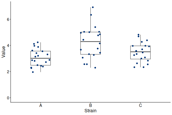
- PDF: width 6 inch and height 4 inch. single-batch_v1.pdf
- Version 2: Colors data points by Strain and adds statistical significance group labels at the top.
- PNG: setting width 600 and height 400.
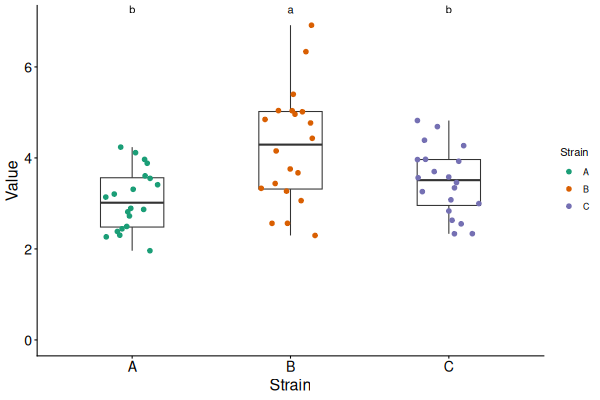
- PDF: width 6 inch and height 4 inch. single-batch_v2.pdf


Multiple batches with replicates
Multiple batches boxplot tutorials
Sample input
R script
- multiple-batches_boxplot.R
# Aim: This R script is about generating multiple batches boxplot.

# Data Description: Multiple batches with replicates
# - sample1.xlsx
#   - Sheet1: Contains raw data across three columns: `Strain`, `Batch`, `Value`. Each strain has three batches.
#   - Sheet2: Contains the statistical test result (Tukey's HSD).
#
# Output (both pdf and png format):
# - Version 1: Displays data with batches shown in distinct colors.
# - Version 2: Displays batches in distinct colors and adds statistical significance group labels at the top.
#---------------------------------------------------------------------------------------------------------------

### Step 0, Check packages

# Required packages
packages <- c("ggplot2", "readxl")

# Check and install required packages
for (pkg in packages) {
  if (!requireNamespace(pkg, quietly = TRUE)) {
    install.packages(pkg, repos = "https://cloud.r-project.org")
  }
}

#---------------------------------------------------------------------------------------------------------------

### Step 1. Configuration

## Set up a dedicated working directory to store your raw files and output plots.

# working directory
working_path = "/scratch/hychang/R_wd/Rana001/Rana001.01/multiple-batches/"

# input data located directory
input_path = "/scratch/hychang/R_wd/Rana001/Rana001.01/multiple-batches/"

# output folder for storing plots
output_path = "/scratch/hychang/R_wd/Rana001/Rana001.01/multiple-batches/plots/"

## Set Input and output

# File name of the raw data table, including the file extension
input_file_raw = "sample2.xlsx"

# Worksheet name of the raw data table
input_sheet_raw = "Sheet1"

# File name of the statistical test result table, including the file extension
input_file_stat = "sample2.xlsx"

# Worksheet name of the statistical test result table
input_sheet_stat = "Sheet2"

# Column names in the input data
x_column = "Strain"
y_column = "Value"
batch_column = "Batch"

# Column name of statistical significance group letters,
# skip if the statistical test not available
stat_column = "groups"

# Output file names of the figures, including the file extension
output_file_1 = "mult-batches_v01.pdf"
output_file_2 = "mult-batches_v02.pdf"
output_file_3 = "mult-batches_v01.png"
output_file_4 = "mult-batches_v02.png"

# Set up a dedicated working directory to store your raw files and output plots.
dir.create(working_path, recursive = TRUE, showWarnings = FALSE)
dir.create(input_path, recursive = TRUE, showWarnings = FALSE)
dir.create(output_path, recursive = TRUE, showWarnings = FALSE)

## Setting figure parameters

# the names of x and y axis
x_lab = "Strain"
y_lab = "Value"

# y axis range and breaks
y_range = c(0, 6)
y_breaks = c(0, 2, 4, 6)

# font size of x and y axis title (axis label)
axis_title_size = 16

# font size of x and y axis text (tick label)
axis_text_size = 14

# sample ordering
x_order = c("A", "B", "C")

# size of data points
point_size= 2

# box size
box_size= 0.4

# space between batches (points)
space_batch = 0.3

# use multiple colors for the data points;
# the number of colors should match the number of batches
color_multiple = c(c("#1B9E77", "#D95F02", "#7570B3"))

## Export setting
pdf_width = 6
pdf_height = 4
png_width = 600
png_height = 400

#---------------------------------------------------------------------------------------------------------------

### Step 2. Setup and Import data

# Set working directory
setwd(working_path)

# load packages
library(readxl)
library(ggplot2)

# Import raw data
df1= read_xlsx(file.path(input_path, input_file_raw), sheet = input_sheet_raw)

# (Optional) Import statistical test result. Skip this step if you don't have the results.
df2= read_xlsx(file.path(input_path, input_file_stat), sheet = input_sheet_stat)

# Sample ordering
df1[[x_column]] = factor(df1[[x_column]], levels = x_order)
df2[[x_column]] = factor(df2[[x_column]], levels = x_order) # skip this if df2 not available

# Display the data frame and view its dimensions (number of rows and columns).
df1; dim(df1)
df2; dim(df2) # skip this if df2 not available

# Show sample counts, including NA values
table(df1[[x_column]], useNA = "always")

# Show the range of values
range(df1[[y_column]])

# check batch counts, including NA values
table(df1[[batch_column]], useNA = "always")
#---------------------------------------------------------------------------------------------------------------

#### Step 3. Generate Plots

# Version 1
# all data points using a single, uniform color.
p1= ggplot(data= df1, aes(x= .data[[x_column]], y= .data[[y_column]]))+
  geom_boxplot(width = box_size,
               outlier.shape = NA)+
  geom_point(data= df1,
             aes(fill= .data[[batch_column]]),
             shape = 21,
             size = point_size,
             position= position_dodge(width = space_batch))+
  scale_fill_manual(values = color_multiple)+
  scale_y_continuous(limits = y_range,
                     breaks = y_breaks)+
  labs(x= x_lab, y= y_lab)+
  theme_classic()+
  theme(axis.title = element_text(size = axis_title_size),
        axis.text = element_text(size = axis_text_size))

# show plot
p1


# Version 2
# colors data points by Strain and adds statistical significance group labels at the top.
p2= ggplot(data = df1, aes(x= .data[[x_column]], y= .data[[y_column]]))+
  geom_boxplot(width = box_size, outlier.shape = NA)+
  geom_point(aes(fill= .data[[batch_column]]),
             shape = 21,
             size = point_size,
             position= position_dodge(width = space_batch))+
  geom_text(data = df2,
            aes(x= .data[[x_column]], y= Inf, label = .data[[stat_column]]),
            vjust= "inward")+
  scale_fill_manual(values = color_multiple)+
  scale_y_continuous(limits = y_range,
                     breaks = y_breaks)+
  labs(x= x_lab, y= y_lab)+
  theme_classic()+
  theme(axis.title = element_text(size = axis_title_size),
        axis.text = element_text(size = axis_text_size))

# show plot
p2


#---------------------------------------------------------------------------------------------------------------
#### Step 4. Export Plots

## Export PDF

# version 1 PDF export
pdf(file.path(output_path, output_file_1), width = pdf_width, height = pdf_height)
p1
dev.off()

# version 2 PDF export
pdf(file.path(output_path, output_file_2), width = pdf_width, height = pdf_height)
p2
dev.off()


## Export PNG

# Version 1 PNG export
png(file.path(output_path, output_file_3), width = png_width, height = png_height)
p1
dev.off()

# Version 2 PNG export
png(file.path(output_path, output_file_4), width = png_width, height = png_height)
p2
dev.off()


### END this script
Sample output
Plots can be exported as PDF or PNG files. Here shows the PNG files.
- Version 1: Displays data with batches shown in distinct colors.
- PNG: setting width 600 and height 400.
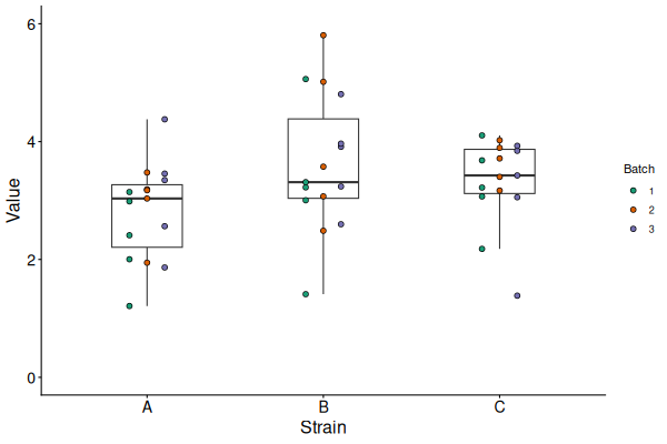
- PDF: width 6 inch and height 4 inch. mult-batches_v01.pdf
- Version 2: Displays batches in distinct colors and adds statistical significance group labels at the top.
- PNG: setting width 600 and height 400.
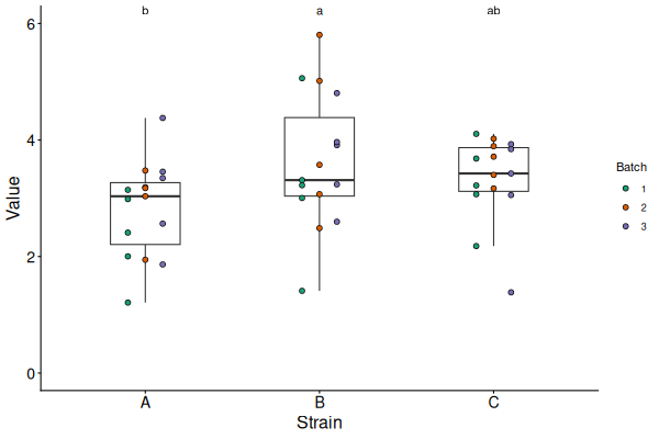
- PDF: width 6 inch and height 4 inch. mult-batches_v02.pdf

